Raster Timeseries Manager

The Raster Timeseries Manager is a plugin for QGIS that allows to navigate through earth observation imagery archives (e.g. Landsat, Sentinel and Modis) and derived products in space and time.

The plugin adds time controls for handling raster layers containing 4D data with two spatial dimensions, one content dimension (e.g. surface reflectance bands and derived features like indices, etc.), and one temporal dimension. Using these time controls, you can navigate and animate observations over time.

A raster timeseries is a normal raster with some additional metadata specified (see Data format).

Layer styling and spatial navigation is handled by QGIS as usual.

Getting started

Installation

In QGIS select QGIS ‣ Plugins ‣ Manage and Install Plugins…, search for RasterTimeseriesManager and install the plugin.

Start

In the toolbar click to show the Raster Timeseries Manager panel.

Load the test data

Select Plugins > Raster Timeseries Manager > Load test data.

Run an animation

In the Raster Timeseries Manager panel select the timeseries layer as current Timeseries.

Click ^{Run Animation}.

Data format

Overview

A timeseries composed of Earth Observation imagery is a regular 4-dimensional data cube:

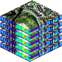
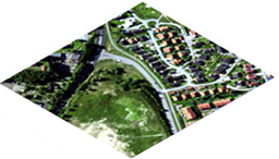
With two spatial dimensions:

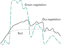
One spectral dimension (e.g. surface reflectance or other derived features like indices):

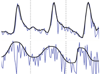
And one temporal dimension:

Binary data

Data is stored as a normal raster in any GDAL supported format (e.g. GTiff, ENVI or VRT).

The raster is a stack of all bands and all observations, thus the content and temporal dimensions are flattened. This is required to match the GDAL data model, which is inherently 3d.

For example, a timeseries of ten Landsat scenes with six reflectance bands each, is stored as a raster stack with 60 bands. The first six bands belong to the first Landsat scene, the next six bands belong to the second Landsat scene, and last six bands belong to the last Landsat scene.

Metadata

Specify names, dates and wavelength (optional) items in the TIMESERIES metadata domain.

All dates must be specified in the yyyy-MM-dd format and wavelength must be specified in Nanometers.

For the test data it looks like this:

/rastertimeseriesmanager/testdata/timeseries.bsq.aux.xml

<PAMDataset>
  <Metadata domain="TIMESERIES">
    <MDI key="names">{blue, green, red, nir, swir1, swir2}</MDI>
    <MDI key="dates">{1984-04-16, 1984-05-09, 1984-05-25, 1984-06-03, 1984-06-10, 1984-06-19, 1984-06-26, 1984-07-22, 1984-08-07, 1984-08-14}</MDI>
    <MDI key="wavelength">{483, 563, 655, 865, 1610, 2200}</MDI>
  </Metadata>
</PAMDataset>

Tip

How to edit metadata:

1. You can manually create/edit the GDAL PAM (Persitant Auxiliary Metadata) sidecar file *.aux.xml with any text editor.

2. You can use the GDAL API. Note that for some raster formats, GDAL stores the metadata inside the raster file, without creating a *.aux.xml sidecar file:

from osgeo import gdal

ds = gdal.Open(filename)
ds.SetMetadataItem('names', '{blue, green, red, nir, swir1, swir2}', 'TIMESERIES')
ds.SetMetadataItem('dates', '{1984-04-16, 1984-05-09, 1984-05-25, 1984-06-03, 1984-06-10, 1984-06-19, 1984-06-26, 1984-07-22, 1984-08-07, 1984-08-14}', 'TIMESERIES')
ds.SetMetadataItem('wavelength', '{483, 563, 655, 865, 1610, 2200}', 'TIMESERIES')
ds = None

Creating a timeseries

It can be very efficient to create a GDAL Virtual Raster File (VRT format) to specify the timeseries without duplicating the data. Virtual Raster Files can be used for raster mosaicking and stacking.

Additionally, for larger mosaics with lots of individual rasters, it is recommended to build overviews. See gdalbuildvrt and gdaladdo.

Also note the Geoserver on steroids talk about preparing large scale raster data for efficient visualisation.

Usage instructions

Basic controls

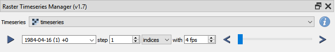
In the Raster Timeseries Manager panel select a Timeseries layer.

Click ^{Run Animation} to start animating the timeseries and to stop.

The : sup:Target date (timeseries observation) +/- days off between target date and timeseries observation widget is updating during animation, but can also be used to select a target date manually and jump to the nearest observation in the timeseries.

Use the step and ^{Step unit} widgets to define how to step through the timeseries, and specify the fps to define the animation speed (note that the actual displayed frames per second depends on the system performance).

Use the ^{Timeseries observation selector} to quickly navigate through the observations.

Advanced Options

Temporal Tab

You can select a start and end date for the animation and specify how to snap from the target date to an actual observation.

Activate the max offset widgets to not show observations that are to far away from the target date. An offset of 0 days would only show the observation if the observation date exactly matches the target date.

Additional TS Tab

Select addition timeseries to be controlled.

Video Creator Tab

In the Video Creator Tab you can grab the animation frames and create MP4 videos and animated GIFs.

1. Make sure that the output folder is empty. You may use the ^{Remove all files from output folder} button.

2. Click ^{Grab frames and store as PNG files}.

3. Click or to create a MP4 video or an animated GIF from the previousely grabed frames.

   Note

   You have to properly setup the external programs FFmpeg and ImageMagick in the System Tab.

   Tip

   You can also use external programs like FFmpeg and ImageMagick directly to create a MP4 or GIF outside of QGIS. For example see: https://trac.ffmpeg.org/wiki/Slideshow

System Tab

To create a MP4 video or an animated GIF you have to install ImageMagick and properly select the FFmpeg and ImageMagick binaries.

Under Windows the default locations are somewhere here:

C:\Program Files\ImageMagick-7.0.3-Q16\ffmpeg.exe
C:\Program Files\ImageMagick-7.0.3-Q16\magick.exe

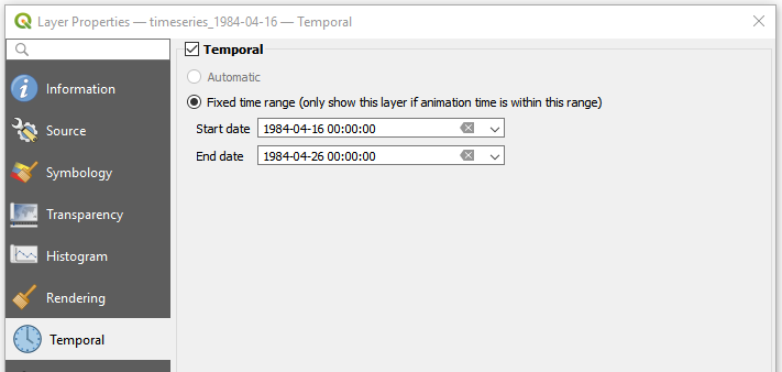
Export Tab

You can export the current timeseries to the QGIS Temporal Controller. For each observation a new raster layer with properly defined temporal properties is created and ready to be used in the QGIS Temporal Controller. The start date is set to the observation date and the end date is set to the observation date plus the fade out time.

Examples

Tasseled Cap Timeseries for whole Turkey

Tasseled Cap Brightness, Greenness and Wetness components for the whole area of Turkey in native 30m Landsat resolution, in 8 day steps for 2015. The dataset is presented in:

Rufin, P., Frantz, D., Ernst, S., Rabe, A., Griffiths, P., Özdoğan, M., & Hostert, P. (2019). Mapping Cropping Practices on a National Scale Using Intra-Annual Landsat Time Series Binning. Remote Sensing, 11, 232. https://doi.org/10.3390/rs11030232

Get in contact (andreas.rabe@geo.hu-berlin.de) if you want to use the dataset (~7 GB).

Example animation zoomed in to native 30 m Landsat resolution

Example animation zoomed to full extent

Enhanced Vegetation Index (EVI) Timeseries for the entire Brazilian savanna

Time series of the Enhanced Vegetation Index (EVI) for the entire Brazilian savanna

The time series covers the entire extent of the Cerrado with Landsat’s native resolution of 30 m x 30 m. The EVI values were derived from Landsat 7 and Landsat 8 observations that were acquired between April 2013 and June 2017. Data gaps in the time series were filled with an ensemble of radial basis convolution filters.

Get in contact (andreas.rabe@geo.hu-berlin.de) if you want to use the dataset (~50 GB).

Example animation zoomed in to native 30 m Landsat resolution

Example animation zoomed to full extent

Contact

Please provide feedback to Andreas Rabe (andreas.rabe@geo.hu-berlin.de) or create an issue.